Water quality

Sep, 2025

Data Analysis

Background

Within the open data catalog of the Basque Government, there is an API available to access information on drinking water (Drinking Water Quality API), and I thought it might be interesting to take a look at it to see whether it could be useful to know something about the water that comes out of our taps.

After exploring the parameter data a bit, I realized that the analysis I should carry out in this project was not so much about interpreting what those data meant (since I lack expertise in the subject), but rather about making a comparison between the values obtained from different measurement points. I decided to compare the water in my hometown, which reaches my house, with that from the largest reservoir in the capital, San Sebastián, which supplies most of the city. This way, I might be able to draw some comparative conclusions about the characteristics of the water.

The data

I wrote some helper classes and functions to:

1. Retrieve the available sampling points for a given municipality.

2. Retrieve the available measurements for a specific sampling point.

3. Retrieve the analytical data obtained in a measurement.

Show code cell source Hide code cell source

import pandas as pd
import matplotlib.pyplot as plt
import seaborn as sns
# Class for this project
from wq_api import WaterQuality

# Instantiate object to access API
wq = WaterQuality()

# Function definition
def sampling_points(county_id, municipality_id, itemsOfPage=100):
    '''Return dataframe with sampling points for municipality.
    '''
    spoints = wq.find_sampling_points(county_id, municipality_id, itemsOfPage=100)

    ids = [item["id"] for item in spoints["items"]]
    names = [item["name"] for item in spoints["items"]]
    zones = [item["location"]["zone"] for item in spoints["items"]]
    
    lenghts, mdates, qcodes = [], [], []
    for id_ in ids:
        measurements = wq.get_measurements(id_)
        lenghts.append(len(measurements))
        dates, codes = [], []
        for measurement in measurements:
            dates.append(measurement["measurementDate"])
            codes.append(measurement["qualificationCode"])
        mdates.append(dates)
        qcodes.append(codes)
    
    points = pd.DataFrame({"id": ids,
                           "name": names,
                           "zone": zones,
                           "measurements": lenghts,
                           "dates": mdates,
                           # "codes": qcodes,
                          })
    
    return points.sort_values(by="measurements", ascending=False)

# Function definition
def dates(point_id, points_df):
    '''Return list of available sampling dates.
    '''
    return list(points_df.loc[points_df["id"] == int(point_id), "dates"])[0]

# Function definition
def analytical_data(point_id, dates):
    '''Return dataframe with available analytical data for sample point.
    '''
    dfs = []
    for date in dates:
        params, values = [], []
        for item in wq.get_analytical_data(point_id, date):
            params.append(item["parameter"] + " (" + item["unitOfMeasure"] + ")")
            values.append(item["value"])
        dfs.append(pd.DataFrame({date: values}, index=params))
    
    return pd.concat(dfs, axis=1)

Get municipality ids for Urretxu and San Sebastian:

Show code cell source Hide code cell source

municipality_ids = pd.read_csv("data/gipuzkoa_ids.csv", index_col="municipality")

urretxu_id = municipality_ids.loc["Urretxu", "id"]
ss_id = municipality_ids.loc["Donostia / San Sebastián", "id"]

print("Municipality ids:")
print(f"- Urretxu -> {urretxu_id}")
print(f"- Donostia / San Sebastián -> {ss_id}")

Municipality ids:
- Urretxu -> 77
- Donostia / San Sebastián -> 69

Show code cell source Hide code cell source

points_ur = sampling_points(county_id="20", # Gipuzkoa
                            municipality_id=urretxu_id)
print("SAMPLING POINTS FOR URRETXU:")
points_ur

SAMPLING POINTS FOR URRETXU:

	id	name	zone	measurements	dates
5	20032077004	ERRATZU DEPOSITOA IRTEERA	BARRENDIOLA	31	[2025-03-18, 2025-02-18, 2025-02-04, 2024-12-1...
6	20032077005	ETXABURU DEPOSITOA IRTEERA	BARRENDIOLA	5	[2025-01-28, 2024-12-17, 2024-02-15, 2023-12-1...
9	20066077001	ERRATZU INDUSTRIALDEA	URRETXU-ZULOAGA	4	[2025-02-18, 2024-12-17, 2024-01-31, 2023-03-16]
4	20032077003	IPIÑARRIETA KALEA	BARRENDIOLA	3	[2025-03-18, 2024-02-28, 2023-03-28]
1	20066077000	ZULOAGA DEPOSITOA IRTEERA	URRETXU-ZULOAGA	2	[2024-08-20, 2023-08-16]
2	20032077001	MUNDO MEJOR	BARRENDIOLA	2	[2024-06-26, 2023-07-05]
0	20032077000	IPARRAGIRRE KALEA	BARRENDIOLA	1	[2023-03-16]
3	20032077002	GERNIKAKO ARBOLA	BARRENDIOLA	1	[2023-03-22]
7	20032077006	INSTITUTO IPARRAGIRRE	BARRENDIOLA	1	[2023-03-21]
8	20032077007	CEMENTERIO	BARRENDIOLA	1	[2023-04-27]
10	20066077002	Deposito Agerre	URRETXU-ZULOAGA	0	[]

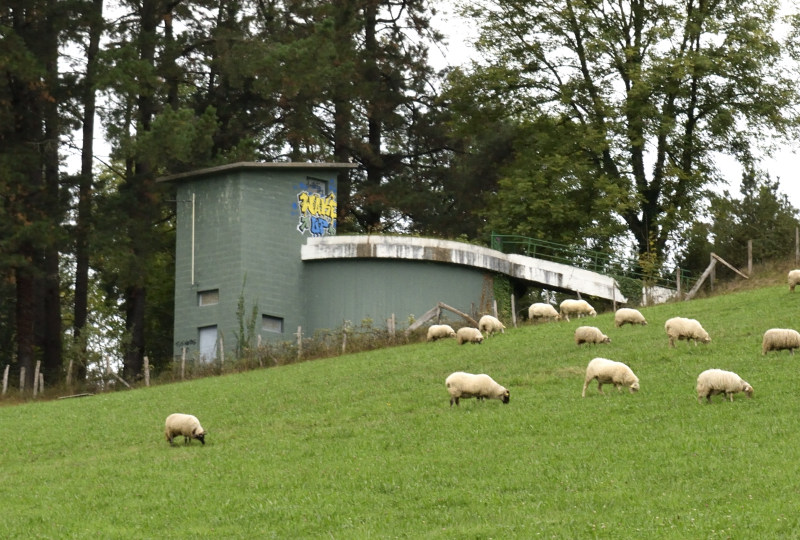
Urretxu has two different drinking water zones: the main one, supplied by the Barrendiola reservoir, and another serving rural areas at higher elevations than the local reservoirs fed by Barrendiola. The main sampling point—with the largest number of measurements—is located at the Erratzu local reservoir, a 1,600 m³ tank that supplies the entire town.

Show code cell source Hide code cell source

points_ss = sampling_points(county_id="20", # Gipuzkoa
                            municipality_id=ss_id)
print("SAMPLING POINTS FOR DONOSTIA / SAN SEBASTIÁN:")
points_ss

SAMPLING POINTS FOR DONOSTIA / SAN SEBASTIÁN:

	id	name	zone	measurements	dates
69	20134069143	DPT. AMARA	AÑARBE	44	[2024-12-27, 2024-11-22, 2024-11-08, 2024-10-2...
0	20134069000	Depósito de Putzueta	AÑARBE	42	[2025-01-03, 2024-12-18, 2024-11-19, 2024-11-0...
77	20134069153	Deposito ORIABENTA Nuevo - Salida	AÑARBE	40	[2024-12-27, 2024-12-13, 2024-11-22, 2024-11-0...
1	20134069100	DEPOSITO MATIA	AÑARBE	39	[2024-12-17, 2024-11-18, 2024-11-05, 2024-10-2...
17	20134069038	DPT. MONS	AÑARBE	39	[2024-12-19, 2024-11-21, 2024-10-24, 2024-10-1...
...	...	...	...	...	...
47	20134069114	Polígono Zuatzu	AÑARBE	0	[]
46	20134069113	FEDERICO GARCIA LORCA	AÑARBE	0	[]
34	20134069086	ZONA ALTA LOIOLA	AÑARBE	0	[]
35	20134069087	ZABALEGUI	AÑARBE	0	[]
89	20134069167	CARCEL MARTUTENE	AÑARBE	0	[]

90 rows × 5 columns

Amara is the main reservoir in San Sebastián, with a capacity of 26,000 m³—about 16 times larger than Urretxu’s largest reservoir, Erratzu.

For the comparison, I will use the available analytical data from:

• Erratzu (20032077004), in Urretxu

• Amara (20134069143), in Donostia / San Sebastián

Show code cell source Hide code cell source

erratzu = "20032077004"
data_erratzu = analytical_data(point_id=erratzu,
                               dates=dates(erratzu, points_ur),
                              )
print("ANALYTICAL DATA IN ERRATZU (URRETXU):")
data_erratzu

ANALYTICAL DATA IN ERRATZU (URRETXU):

	2025-03-18	2025-02-18	2025-02-04	2024-12-17	2024-11-20	2024-11-12	2024-11-06	2024-10-22	2024-09-25	2024-08-20	...	2023-06-20	2023-06-14	2023-05-15	2023-04-24	2023-03-28	2023-03-22	2023-03-16	2023-03-13	2023-02-13	2023-01-23
AMONIO (mg/l)	0.00	0.00	0.00	0.00	0.00	0.00	0.00	0.05	0.05	0.05	...	0.05	0.10	0.10	0.10	0.05	0.05	0.05	0.1	0.10	0.10
CLORO LIBRE RESIDUAL (mg/l)	0.43	0.59	0.56	0.39	0.37	0.33	0.39	0.43	0.35	0.33	...	0.42	0.69	0.81	0.83	0.54	0.48	0.47	0.8	0.75	0.85
COLIFORMES TOTALES (ufc/100 ml)	0.00	0.00	0.00	0.00	0.00	0.00	0.00	0.00	0.00	0.00	...	0.00	0.00	0.00	0.00	0.00	0.00	0.00	0.0	0.00	0.00
COLOR (Pt/Co) (mg/l)	0.00	0.00	0.00	0.00	0.00	0.00	7.00	4.00	4.00	4.00	...	4.00	5.00	5.00	5.00	4.00	4.00	4.00	5.0	5.00	5.00
CONDUCTIVIDAD (20ºC) (µs/cm)	123.00	118.00	117.00	121.00	136.00	130.00	133.00	142.00	140.00	129.00	...	136.00	130.00	124.00	123.00	122.00	122.00	122.00	120.0	119.00	121.00
...	...	...	...	...	...	...	...	...	...	...	...	...	...	...	...	...	...	...	...	...	...
SULFATO (mg/l)	NaN	NaN	NaN	NaN	NaN	NaN	NaN	NaN	NaN	NaN	...	NaN	NaN	NaN	NaN	NaN	NaN	12.00	NaN	NaN	NaN
TETRACLOROETENO (µg/l)	NaN	NaN	NaN	NaN	NaN	NaN	NaN	NaN	NaN	NaN	...	NaN	NaN	NaN	NaN	NaN	NaN	0.50	NaN	NaN	NaN
TRICLOROETENO (µg/l)	NaN	NaN	NaN	NaN	NaN	NaN	NaN	NaN	NaN	NaN	...	NaN	NaN	NaN	NaN	NaN	NaN	0.50	NaN	NaN	NaN
TRICLOROETENO+TETRACLOROETENO (µg/l)	NaN	NaN	NaN	NaN	NaN	NaN	NaN	NaN	NaN	NaN	...	NaN	NaN	NaN	NaN	NaN	NaN	0.50	NaN	NaN	NaN
TRIHALOMETANOS(THMS) (µg/l)	NaN	NaN	NaN	NaN	NaN	NaN	NaN	NaN	NaN	NaN	...	NaN	NaN	NaN	NaN	NaN	NaN	6.00	NaN	NaN	NaN

93 rows × 31 columns

Show code cell source Hide code cell source

amara = "20134069143"
data_amara = analytical_data(point_id=amara,
                             dates=dates(amara, points_ss),
                            )
print("ANALYTICAL DATA IN AMARA (DONOSTIA / SAN SEBASTIÁN):")
data_amara

ANALYTICAL DATA IN AMARA (DONOSTIA / SAN SEBASTIÁN):

	2024-12-27	2024-11-22	2024-11-08	2024-10-25	2024-09-27	2024-09-16	2024-08-23	2024-07-26	2024-06-28	2024-06-14	...	2023-05-26	2023-05-05	2023-04-28	2023-04-14	2023-03-24	2023-03-10	2023-02-24	2023-02-10	2023-01-27	2023-01-13
ALCALINIDAD (HC03) (mg/l)	47.40	44.40	45.50	40.50	45.10	41.80	47.20	43.90	42.30	43.20	...	39.700	44.80	47.80	49.20	49.90	50.00	44.80	47.10	47.80	42.80
ALUMINIO (µg/l)	34.00	49.50	54.30	43.40	53.20	50.30	50.30	52.50	40.10	42.80	...	34.500	24.80	40.50	31.90	39.50	27.50	33.00	32.00	33.00	37.00
CALCIO (mg/l)	20.70	20.00	20.00	18.90	19.30	17.50	19.30	18.90	19.10	19.40	...	18.600	19.50	19.90	21.70	20.80	21.80	19.20	20.30	20.80	18.10
CLORO LIBRE RESIDUAL (mg/l)	0.65	0.66	0.61	0.67	0.59	0.49	0.62	0.68	0.59	0.65	...	0.810	0.77	0.75	0.76	0.71	0.68	0.66	0.61	0.70	0.55
COLIFORMES TOTALES (ufc/100 ml)	0.00	0.00	0.00	0.00	0.00	0.00	0.00	0.00	0.00	0.00	...	0.000	0.00	0.00	0.00	0.00	0.00	0.00	0.00	0.00	0.00
COLOR (Pt/Co) (mg/l)	0.00	0.00	0.00	0.00	3.00	3.00	3.00	3.00	3.00	3.00	...	3.000	3.00	3.00	3.00	3.00	3.00	3.00	3.00	3.00	3.00
CONDUCTIVIDAD (20ºC) (µs/cm)	131.00	127.00	129.00	122.00	122.00	118.00	124.00	119.00	119.00	119.00	...	127.000	123.00	126.00	131.00	134.00	131.00	135.00	130.00	137.00	122.00
DUREZA TOTAL CALCIO (CaCO3) (mg/l)	58.00	56.00	56.00	53.00	53.00	49.00	54.00	52.00	53.00	53.00	...	52.000	54.00	55.00	59.00	57.00	60.00	53.00	56.00	57.00	51.00
ENTEROCOCOS (ufc/100 ml)	0.00	0.00	0.00	0.00	0.00	0.00	0.00	0.00	0.00	0.00	...	0.000	NaN	NaN	NaN	NaN	NaN	NaN	NaN	NaN	NaN
ESCHERICHIA COLI (ufc/100 ml)	0.00	0.00	0.00	0.00	0.00	0.00	0.00	0.00	0.00	0.00	...	0.000	0.00	0.00	0.00	0.00	0.00	0.00	0.00	0.00	0.00
HIERRO (µg/l)	0.00	0.00	0.00	0.00	5.00	5.00	5.00	5.00	5.00	5.00	...	5.000	5.00	5.00	5.00	5.00	5.00	5.00	5.00	5.00	5.00
INDICE DE LANGELIER (-)	-1.30	-1.30	-1.30	-1.10	-1.80	-1.90	NaN	NaN	NaN	NaN	...	NaN	NaN	NaN	NaN	NaN	NaN	NaN	NaN	NaN	NaN
MAGNESIO (mg/l)	1.43	1.38	1.41	1.38	1.28	1.27	1.45	1.04	1.21	1.17	...	1.410	1.23	1.19	1.11	1.28	1.30	1.14	1.27	1.26	1.31
MANGANESO (µg/l)	0.00	0.00	0.00	0.00	2.50	2.50	2.50	2.50	2.50	2.50	...	2.500	2.50	2.50	2.50	2.50	2.50	2.50	2.50	2.50	2.50
PH (20ºC) (-)	7.60	7.70	7.70	7.30	7.70	7.30	7.60	7.60	7.50	7.60	...	7.430	7.60	7.49	7.71	7.55	7.56	7.57	7.59	7.58	7.63
RECUENTO DE BACTERIAS HETEROTROFAS A 22ºC (ufc/ml)	0.00	0.00	0.00	0.00	1.00	1.00	1.00	1.00	1.00	1.00	...	1.000	1.00	1.00	1.00	1.00	1.00	1.00	1.00	1.00	1.00
TEMPERATURA (ºc)	12.10	15.20	16.10	16.30	16.90	15.70	15.30	15.10	15.80	13.90	...	11.600	10.80	10.50	9.90	9.90	9.30	9.40	9.10	9.80	11.20
TURBIDEZ (unf)	0.00	0.00	0.00	0.00	0.25	0.25	0.25	0.25	0.25	0.25	...	0.106	0.10	0.10	0.10	0.10	0.10	0.10	0.10	0.10	0.10
COLIFORMES TOTALES (NMP) (nmp/100 ml)	NaN	NaN	NaN	NaN	NaN	NaN	NaN	NaN	NaN	NaN	...	NaN	NaN	NaN	NaN	NaN	NaN	NaN	NaN	NaN	NaN
ESCHERICHIA COLI (NMP) (nmp/100 ml)	NaN	NaN	NaN	NaN	NaN	NaN	NaN	NaN	NaN	NaN	...	NaN	NaN	NaN	NaN	NaN	NaN	NaN	NaN	NaN	NaN
ESTREPTOCOCOS FECALES (nmp/ 100 ml)	NaN	NaN	NaN	NaN	NaN	NaN	NaN	NaN	NaN	NaN	...	NaN	NaN	NaN	NaN	NaN	NaN	NaN	NaN	NaN	NaN
AMONIO (mg/l)	NaN	NaN	NaN	NaN	NaN	NaN	NaN	NaN	NaN	NaN	...	NaN	NaN	0.05	0.05	0.05	0.05	0.05	0.05	0.05	0.05
CLOSTRIDIUM PERFRINGENS (INCLUIDAS LAS ESPORAS) (ufc/100 ml)	NaN	NaN	NaN	NaN	NaN	NaN	NaN	NaN	NaN	NaN	...	NaN	NaN	0.00	0.00	0.00	0.00	0.00	0.00	0.00	0.00
NITRITOS (mg/l)	NaN	NaN	NaN	NaN	NaN	NaN	NaN	NaN	NaN	NaN	...	NaN	NaN	0.01	0.01	0.01	0.01	0.01	0.01	0.01	0.01
RECUENTO DE BACTERIAS HETEROTROFAS A 37ºC (ufc/ml)	NaN	NaN	NaN	NaN	NaN	NaN	NaN	NaN	NaN	NaN	...	NaN	NaN	1.00	1.00	1.00	2.00	1.00	1.00	1.00	1.00

25 rows × 44 columns

Data analysis

Available parameters

Let’s first get a comparative view of available parameters and the number of times they were sampled in each of the reservoirs:

Show code cell source Hide code cell source

# Compute each parameter quantities
samples_erratzu = data_erratzu.notna().sum(axis=1)
samples_erratzu = samples_erratzu.sort_values(ascending=False).to_frame(name="erratzu")

samples_amara = data_amara.notna().sum(axis=1)
samples_amara = samples_amara.sort_values(ascending=False).to_frame(name="amara")

# Get all of them in one dataframe
samples_all = samples_amara.join(samples_erratzu, how="outer")
samples_all = samples_all.sort_values("amara", ascending=False)

# Plot
fig, ax = plt.subplots(figsize=(8, 16))
samples_all.plot(ax=ax, kind="barh")
ax.invert_yaxis()
ax.grid(axis="x", alpha=0.3)
ax.set_axisbelow(True)
ax.set_title("Available parameters", size=11)
ax.set_xlabel("Number of samples")
ax.tick_params(axis='y', labelsize=8, rotation=0)
sns.despine()
plt.show()

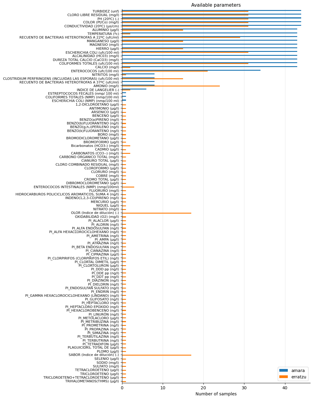
The available measurements for Amara appear more consistent in the parameters that are regularly monitored. In Erratzu, there was one measurement where many parameters were sampled, but it occurred only once.

Show code cell source Hide code cell source

# Compute number of parameters sampled by date
dates_erratzu = data_erratzu.notna().sum()
dates_erratzu = dates_erratzu.sort_index().to_frame(name="erratzu")

dates_amara = data_amara.notna().sum()
dates_amara = dates_amara.sort_index().to_frame(name="amara")

# Get all of them in one dataframe
dates_all = dates_amara.join(dates_erratzu, how="outer")
dates_all.index = pd.to_datetime(dates_all.index)

# Plot
fig, ax = plt.subplots(figsize=(6, 4))
ax.plot(dates_all.index, dates_all["amara"], ".", label="amara")
ax.plot(dates_all.index, dates_all["erratzu"], ".", label="erratzu")
ax.vlines(dates_all.index, ymin=0, ymax=dates_all["amara"], linestyle="-", alpha=0.7)
ax.vlines(dates_all.index, ymin=0, ymax=dates_all["erratzu"], linestyle="-", alpha=0.7,
          color=sns.color_palette("tab10")[1])
ax.grid(axis="y", alpha=0.3)
ax.set_axisbelow(True)
ax.set_ylim(0)
ax.set_title("Number of parameters sampled by date", size=11)
ax.set_ylabel("Number of parameters")
for i in range(2023, 2026):
    ax.axvline(pd.to_datetime(str(i)), linestyle="--", color="grey", linewidth=0.5)
fig.autofmt_xdate()
ax.legend()
sns.despine()
plt.show()

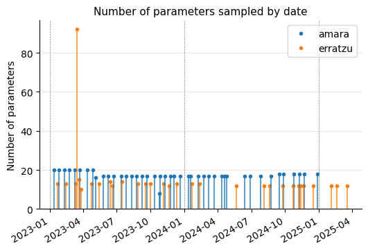
As we can see, data is available from 2023 onward, and lately the frequency of measurements (or at least the data provided through the API) appears to be more limited. Typically, more parameters are measured in Amara than in Erratzu.
The graph also clearly shows that, in Erratzu, there was one occasion (2023-03-16) where a large number of parameters were sampled. Is this an indication than some parameters where found to be out of range previously? I will show this date in the following graphs as a vertical line for reference.

Comparison

As mentioned earlier, this project will focus solely on a comparative analysis, so I will only plot parameters that have been sampled in both reservoirs at least once.

Show code cell source Hide code cell source

# Perform an inner merge to get parameters in both
samples_both = samples_amara.join(samples_erratzu, how="inner")
samples_both

	amara	erratzu
TURBIDEZ (unf)	44	31
CLORO LIBRE RESIDUAL (mg/l)	44	31
COLOR (Pt/Co) (mg/l)	44	31
CONDUCTIVIDAD (20ºC) (µs/cm)	44	31
PH (20ºC) (-)	44	31
ALUMINIO (µg/l)	43	15
TEMPERATURA (ºc)	43	2
RECUENTO DE BACTERIAS HETEROTROFAS A 22ºC (ufc/ml)	43	29
MANGANESO (µg/l)	43	15
HIERRO (µg/l)	43	15
ESCHERICHIA COLI (ufc/100 ml)	43	31
COLIFORMES TOTALES (ufc/100 ml)	43	31
CALCIO (mg/l)	43	2
ENTEROCOCOS (ufc/100 ml)	34	21
AMONIO (mg/l)	8	24
CLOSTRIDIUM PERFRINGENS (INCLUIDAS LAS ESPORAS) (ufc/100 ml)	8	15
NITRITOS (mg/l)	8	1
INDICE DE LANGELIER (-)	6	2

Show code cell source Hide code cell source

# Subset dataframe with data for common parameters
data_amara_common = data_amara[data_amara.index.isin(samples_both.index)]
data_amara_common_t = data_amara_common.transpose().sort_index()
data_amara_common_t.index = pd.to_datetime(data_amara_common_t.index)

data_erratzu_common = data_erratzu[data_erratzu.index.isin(samples_both.index)]
data_erratzu_common_t = data_erratzu_common.transpose().sort_index()
data_erratzu_common_t.index = pd.to_datetime(data_erratzu_common_t.index)

# Define plot function
def plot_params(params):
    for param in params:
        fig, ax = plt.subplots(figsize=(6, 4))
        data_amara_common_t[[param]].plot(ax=ax, marker=".", linewidth=0.5)
        data_erratzu_common_t[[param]].plot(ax=ax, marker=".", linewidth=0.5)
        ax.grid(axis="both", alpha=0.3)
        ax.set_axisbelow(True)
        ax.set_title(param, size=10)
        fig.autofmt_xdate()
        h, l = ax.get_legend_handles_labels()
        ax.legend(handles=h, labels=["amara", "erratzu"])
        ax.axvline("2023-03-16", linestyle="--", color="grey", linewidth=0.5)
        sns.despine()
        plt.show()

Parámetros Físicos y Organolépticos

Estos afectan la apariencia, sabor y olor del agua, más que la salud directa (aunque altos niveles pueden indicar problemas subyacentes). Interesantes si el agua “no parece potable” (ej. turbia o con mal olor).

Parámetro	Descripción	Rango indicado para consumo humano
PH (20ºC)	Mide acidez/alcalinidad; afecta corrosión y sabor.	Ideal 6.5-9.5; fuera de rango puede indicar contaminación o problemas en tratamiento.
COLOR (Pt/Co)	Indica impurezas orgánicas o minerales.	Debe ser bajo (<5 Pt/Co) para aceptabilidad; alto puede ser inofensivo pero desagradable.
TURBIDEZ	Mide claridad; alto puede ocultar patógenos.	<1 NTU para desinfección efectiva y estética.
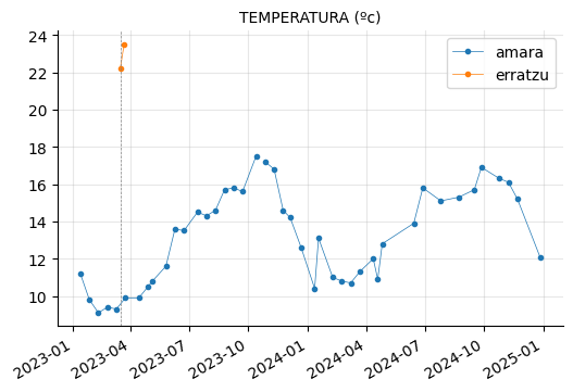
TEMPERATURA	Afecta crecimiento bacteriano y sabor.	<25ºC es preferible para consumo.

Show code cell source Hide code cell source

params_1 = ["PH (20ºC) (-)",
            "COLOR (Pt/Co) (mg/l)",
            "TURBIDEZ (unf)",
            "TEMPERATURA (ºc)"]

plot_params(params_1)

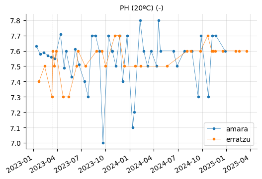
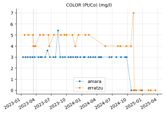
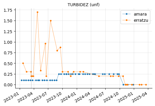
Erratzu appears to have had issues with COLOR and TURBIDEZ, although these parameters seem to have returned to normal in the most recent measurements.

Parámetros Químicos Inorgánicos y Metales

Estos miden sales, metales y nutrientes. Interesantes para estudiar dureza del agua (afecta electrodomésticos) o toxicidad crónica (ej. metales pesados). Muchos tienen límites por salud a largo plazo.

Parámetro	Descripción	Rango indicado para consumo humano
CONDUCTIVIDAD (20ºC)	Mide sales totales; indica mineralización.	<2500 µS/cm; alto puede sugerir contaminación salina.
AMONIO	De descomposición orgánica; alto indica contaminación.	<0.5 mg/L; puede formar compuestos tóxicos con cloro.
ALUMINIO / HIERRO / MANGANESO	Metales de sedimentos o corrosión.	alto aluminio (>0.2 mg/L) o hierro (>0.2 mg/L) afectan salud.
CALCIO / BICARBONATOS (HCO3-) / CARBONATOS (CO3–)	Componentes de dureza; índice de Langelier evalúa corrosión.	indican si el agua es “”dura”” (puede formar incrustaciones).
NITRATO / NITRITOS	De fertilizantes; altos causan metahemoglobinemia.	nitrato <50 mg/L, nitritos <0.5 mg/L; críticos para bebés.

Show code cell source Hide code cell source

params_2 = ["CONDUCTIVIDAD (20ºC) (µs/cm)",
            "AMONIO (mg/l)",
            "ALUMINIO (µg/l)", "HIERRO (µg/l)", "MANGANESO (µg/l)",
            "CALCIO (mg/l)", "INDICE DE LANGELIER (-)",
            "NITRITOS (mg/l)"]

plot_params(params_2)

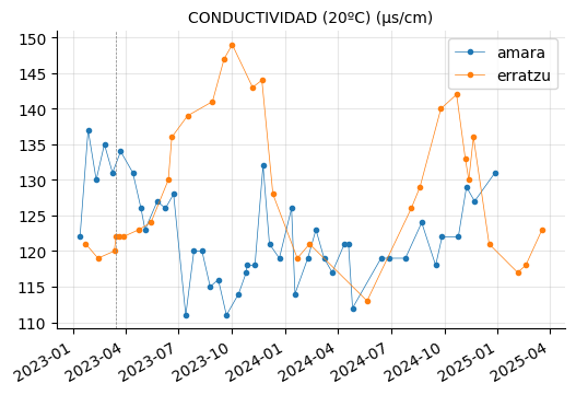
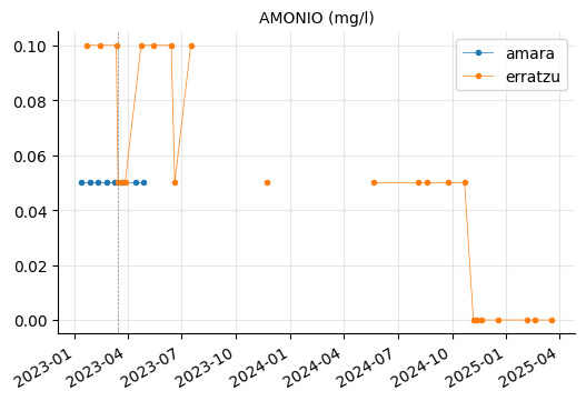
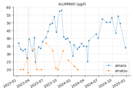
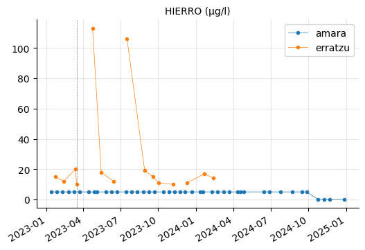
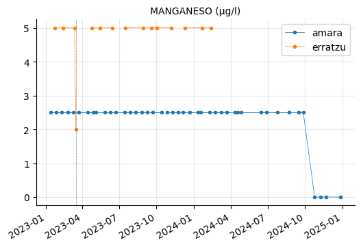
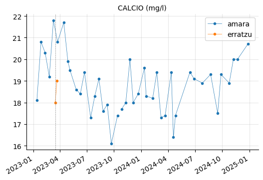
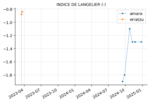
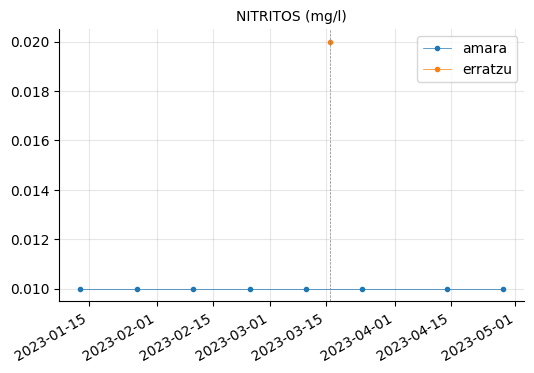
ALUMINIO, HIERRO, and MANGANESO levels tend to vary between the reservoirs, but they do not appear to be out of range.

Parámetros Microbiológicos

Estos son críticos porque indican contaminación fecal o patógenos que pueden causar enfermedades. Son esenciales para evaluar si el agua es segura para beber. Interesantes para estudiar si hay sospechas de contaminación (ej. por roturas en tuberías).

Parámetro	Descripción	Rango indicado para consumo humano
COLIFORMES TOTALES	Detecta bacterias indicadoras de contaminación.	debe estar ausente o muy bajo; alto nivel sugiere riesgo sanitario.
ESCHERICHIA COLI	Indicador específico de contaminación fecal reciente.	debe ser 0 UFC/100 ml para potabilidad.
RECUENTO DE BACTERIAS HETEROTROFAS A 22ºC	Mide bacterias generales en el agua.	indica estabilidad biológica; alto puede sugerir biofilm en tuberías.
ENTEROCOCOS / ENTEROCOCOS INTESTINALES (NMP)	Indicadores de contaminación fecal resistente.	deben estar ausentes; relacionados con infecciones gastrointestinales.
CLOSTRIDIUM PERFRINGENS (INCLUIDAS LAS ESPORAS)	Detecta contaminación antigua o por suelos.	indicador de tratamiento insuficiente; debe ser 0.

Show code cell source Hide code cell source

params_3 = ["COLIFORMES TOTALES (ufc/100 ml)",
            "ESCHERICHIA COLI (ufc/100 ml)",
            "RECUENTO DE BACTERIAS HETEROTROFAS A 22ºC (ufc/ml)",
            "ENTEROCOCOS (ufc/100 ml)",
            "CLOSTRIDIUM PERFRINGENS (INCLUIDAS LAS ESPORAS) (ufc/100 ml)"]

plot_params(params_3)

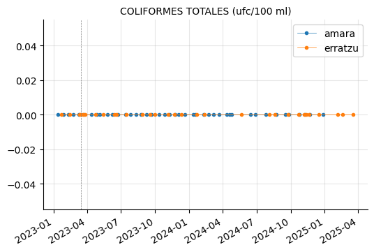
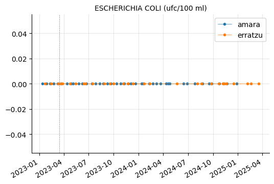
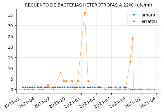
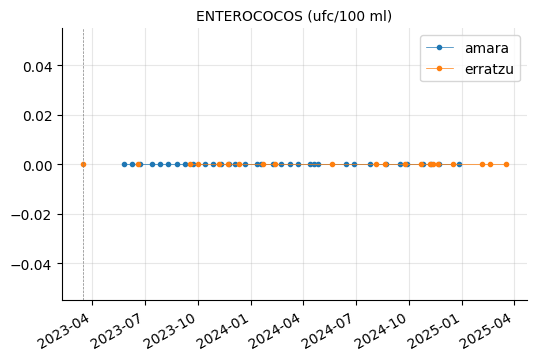
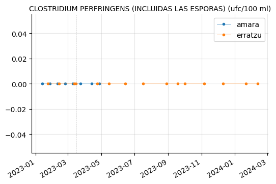
RECUENTO DE BACTERIAS HETEROTROFAS A 22ºC showed a couple of peaks in Erratzu, but the issue seems to have been resolved.

Parámetros Relacionados con Desinfección

Estos evalúan el tratamiento (cloración). Interesantes para balancear desinfección vs. subproductos.

Parámetro	Descripción	Rango indicado para consumo humano
CLORO LIBRE RESIDUAL / CLORO COMBINADO RESIDUAL	Niveles de desinfectante.	0.2-1 mg/L libre; asegura protección bacteriana sin exceso (que causa sabor).

Show code cell source Hide code cell source

params_4 = ["CLORO LIBRE RESIDUAL (mg/l)"]

plot_params(params_4)

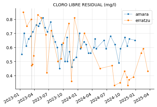
Both are inside recommended range but is there a significant difference in chlorine (CLORO) levels between the two reservoirs? Let’s plot average values with confidence intervals to check it out.

Show code cell source Hide code cell source

# Subset CLORO
cloro_amara = data_amara_common_t["CLORO LIBRE RESIDUAL (mg/l)"].to_frame("amara")
cloro_erratzu = data_erratzu_common_t["CLORO LIBRE RESIDUAL (mg/l)"].to_frame("erratzu")

# Prepare dataframe for seaborn plotting
cloro = cloro_amara.join(cloro_erratzu, how="outer").melt().dropna()

# Plot
fig, ax = plt.subplots(figsize=(6, 4))
sns.pointplot(x="variable", y="value", data=cloro, hue="variable")
ax.grid(axis="both", alpha=0.3)
ax.set_axisbelow(True)
ax.set_title("CLORO LIBRE RESIDUAL, avg. values", size=10)
ax.set_xlabel("")
ax.set_ylabel("mg/L")
ax.axhline(1, color="black", linewidth=0.5)
ax.axhline(0.2, color="black", linewidth=0.5)
ax.annotate("max", (-0.3, 1), size=8)
ax.annotate("min", (-0.3, 0.2), size=8)
sns.despine()
plt.show()

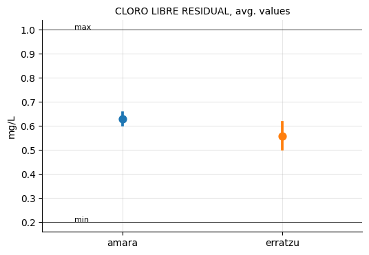
On average, the water from Erratzu seems to be slightly less chlorinated than that from Amara, a result strongly influenced by the most recent measurements, where Erratzu’s values were clearly below Amara’s. However, the difference is minimal, and in any case, both are within the recommended range.

Conclusion

Overall, there do not appear to be significant differences between the characteristics of the drinking water in Erratzu (Urretxu) and Amara (San Sebastián). This is not unexpected, given that although the water originates from different reservoirs (Barrendiola and Añarbe, respectively), the sources are geographically close, and in both cases the water is treated in purification plants before reaching the storage tanks where the measurements were taken.

That said, the scope for comparative analysis is limited by inconsistencies in the selection of analyzed parameters. For example, water hardness is an important parameter, as it affects the lifespan of washing machines and dishwashers and is sometimes necessary to know in order to maintain these appliances properly. While this parameter is consistently measured in Amara, it is not measured in Erratzu. Consequently, it is not included in this study, illustrating the inconsistency in the parameters monitored.