Movie records

\(^{1}\)Photo of the local cinema taken from Zelai Arizti.

Feb, 2024

Data mining with API

Background

For a little over a decade, I’ve been keeping a record of the movies I watch, both in theaters and at home. I jot down the title, director, release year, and rate them with stars based on how I felt about them. In reality, my rating system consists of just two numbers: I give 4 stars if I liked the movie and 5 if I loved it. If a movie didn’t evoke any special feelings, I leave the rating box blank. This dataset now has almost a thousand entries, and I’ve thought about analyzing it to answer some questions I have.

For instance, lately I’ve had the feeling that movies are getting longer. Is this true, or is it just my impression? To get the duration in minutes for each film and integrate it into my table, I thought about using the API of the online movie database TMDB (The Movie Database). Once connected to it, besides the runtime, I could also complete the information, for example, with the ratings received by each movie and compare my tastes with those of the community.

Show code cell source Hide code cell source

# Import basic packages
import numpy as np
import pandas as pd
import matplotlib.pyplot as plt
import seaborn as sns

# TMDB API wrapper
import tmdbsimple as tmdb

# More packages
from iso639 import Lang
import warnings

The data

First I read my records from a CSV file:

Show code cell source Hide code cell source

# Read from file my movie records
films = pd.read_csv('data/films.csv', usecols=['title', 'director', 'year', 'stars'])
films

	title	director	year	stars
0	Inland Empire	David Lynch	2006	4.0
1	La vida es un milagro	Emir Kusturica	2004	NaN
2	El arca rusa	Aleksandr Sokurov	2002	5.0
3	Biutiful	Alejandro Glez. Iñárritu	2010	NaN
4	Carretera perdida	David Lynch	1997	NaN
...	...	...	...	...
928	Anatomía de una caída	Justine Triet	2023	4.0
929	Fallen Leaves	Aki Kaurismäki	2023	4.0
930	Chinas	Arantxa Echevarría	2023	NaN
931	Una habitación con vistas	James Ivory	1985	NaN
932	Els encantats	Elena Trapé	2023	4.0

933 rows × 4 columns

Next, I am going to collect the information to complete the table. To simplify the code and facilitate access, I found the following library for the TMDB API: tmdbsimple. It has a function that utilizes the movie search utility based on its title. In my table, the movie titles are often in Spanish, and this function finds the closest match in the TMBD database. To fine-tune the results, I include the movie’s release year in the search.

Next, once the movie identifier is found, I access the movie record so I can get the following information:

• tmdb_id: film TMDB identifier.

• tmdb_title: title given in TMDB (normaly the English one).

• tmdb_genre: here I filter the response to differentiate between documentaries and just films (fiction films).

• tmdb_lang: original language.

• tmdb_runtime: duration of the film in minutes.

• tmdb_vote_cnt: number of ratings.

• tmdb_vote_avg: average rating.

Show code cell source Hide code cell source

# Init TMDB API parameters
tmdb.API_KEY = "api-key"
tmdb.REQUESTS_TIMEOUT = 5  # seconds, for both connect and read


# ****SEARCH MOVIE****

# Init Search method
search = tmdb.Search()

# Iterate through my records' title and year to find TMDB id
tmdb_ids = []
tmdb_titles = []

for row in range(len(films)):
    
    response = search.movie(query=films.loc[row, 'title'],
                            year=films.loc[row, 'year'])

    # Iterate through the possible movies
    ids = []
    titles = []
    for i in range(len(response['results'])):
        ids.append(response['results'][i]['id'])
        titles.append(response['results'][i]['title'])

    # I will take the most probable film found, first in the list
    try:
        tmdb_ids.append(ids[0])
        tmdb_titles.append(titles[0])
    except:
        tmdb_ids.append("")
        tmdb_titles.append("")


# Assign new columns to the dataframe    
films['tmdb_title'] = tmdb_titles
films['tmdb_id'] = tmdb_ids



# ****GET MOVIE INFO****

# Iterate through the films to fetch the required info
tmdb_genres = []
tmdb_langs = []
tmdb_runtimes = []
tmdb_vote_cnts = []
tmdb_vote_avgs = []

for row in range(len(films)):

    movie = tmdb.Movies(films.loc[row, 'tmdb_id'])

    # Get genres distinguishing Documentaries from Films
    try:
        tmdb_genre = 'Film'
        for genre in movie.info()['genres']:
            if genre['name'] == 'Documentary':
                tmdb_genre = 'Documentary'
        tmdb_genres.append(tmdb_genre)
    except:
        tmdb_genres.append("")

    # Get the language
    try:
        tmdb_langs.append(movie.info()['original_language'])
    except:
        tmdb_langs.append("")

    # Get the runtime
    try:
        tmdb_runtimes.append(movie.info()['runtime'])
    except:
        tmdb_runtimes.append("")

    # Get the rating counts
    try:
        tmdb_vote_cnts.append(movie.info()['vote_count'])
    except:
        tmdb_vote_cnts.append("")

    # Get the rating
    try:
        tmdb_vote_avgs.append(movie.info()['vote_average'])
    except:
        tmdb_vote_avgs.append("")
    

# Assign new columns to the dataframe  
films['tmdb_genre'] = tmdb_genres
films['tmdb_lang'] = tmdb_langs
films['tmdb_runtime'] = tmdb_runtimes
films['tmdb_vote_cnt'] = tmdb_vote_cnts
films['tmdb_vote_avg'] = tmdb_vote_avgs

# Print the resulting dataframe
films

	title	director	year	stars	tmdb_title	tmdb_id	tmdb_genre	tmdb_lang	tmdb_runtime	tmdb_vote_cnt	tmdb_vote_avg
0	Inland Empire	David Lynch	2006	4.0	Inland Empire	1730	Film	en	180	1007	7.023
1	La vida es un milagro	Emir Kusturica	2004	NaN	Life Is a Miracle	20128	Film	sr	155	163	7.365
2	El arca rusa	Aleksandr Sokurov	2002	5.0	Russian Ark	16646	Film	ru	99	425	7.3
3	Biutiful	Alejandro Glez. Iñárritu	2010	NaN	Biutiful	45958	Film	es	148	1040	7.255
4	Carretera perdida	David Lynch	1997	NaN	Lost Highway	638	Film	en	134	2422	7.6
...	...	...	...	...	...	...	...	...	...	...	...
928	Anatomía de una caída	Justine Triet	2023	4.0	Anatomy of a Fall	915935	Film	fr	152	897	7.7
929	Fallen Leaves	Aki Kaurismäki	2023	4.0	Fallen Leaves	986280	Film	fi	81	269	7.258
930	Chinas	Arantxa Echevarría	2023	NaN	Chinas	1034387	Film	es	119	8	7.938
931	Una habitación con vistas	James Ivory	1985	NaN	A Room with a View	11257	Film	en	117	690	6.988
932	Els encantats	Elena Trapé	2023	4.0	The Enchanted	1022725	Film	ca	108	8	6.8

933 rows × 11 columns

Show code cell source Hide code cell source

# Save data into a file
films.to_csv('data/films-tmdb.csv')

# Read from file
films = pd.read_csv('data/films-tmdb.csv', index_col=False)

# Get dataframe info
films.info()

<class 'pandas.core.frame.DataFrame'>
RangeIndex: 933 entries, 0 to 932
Data columns (total 12 columns):
 #   Column         Non-Null Count  Dtype  
---  ------         --------------  -----  
 0   Unnamed: 0     933 non-null    int64  
 1   title          933 non-null    object 
 2   director       933 non-null    object 
 3   year           933 non-null    int64  
 4   stars          176 non-null    float64
 5   tmdb_title     927 non-null    object 
 6   tmdb_id        927 non-null    float64
 7   tmdb_genre     927 non-null    object 
 8   tmdb_lang      927 non-null    object 
 9   tmdb_runtime   927 non-null    float64
 10  tmdb_vote_cnt  927 non-null    float64
 11  tmdb_vote_avg  927 non-null    float64
dtypes: float64(5), int64(2), object(5)
memory usage: 87.6+ KB

Data validation

Missing values in the tmdb_ columns indicate that the film was not found in TMDB, so I discard those rows altogether since there is no information available for them. Furthermore, I adjust the data types for integers (id, runtime, number of ratings) and categorize the genre, language, and the number of stars that I assign. In the latter case, 4 stars become “liked,” 5 stars become “loved,” and missing values are classified as “untagged.”

Show code cell source Hide code cell source

# Drop films that were not found in TMDB
films = films.dropna(subset='tmdb_id')

# Convert to integer data types
films['tmdb_id'] = films['tmdb_id'].astype('int64')
films['tmdb_runtime'] = films['tmdb_runtime'].astype('int64')
films['tmdb_vote_cnt'] = films['tmdb_vote_cnt'].astype('int64')

# Round rating values
films['tmdb_vote_avg'] = round(films['tmdb_vote_avg'], 1)

# Categorize "stars", my personal preferences, as follows
films['stars'] = films['stars'].fillna(0).replace({5: 'loved', 4: 'liked', 0: 'untagged'}).astype('category')

# Categorize genre elements: Film, Documentary.
films['tmdb_genre'] = films['tmdb_genre'].astype('category')

# Categorize languages
films['tmdb_lang'] = films['tmdb_lang'].astype('category')

# Get dataframe info
films.info()

<class 'pandas.core.frame.DataFrame'>
Index: 927 entries, 0 to 932
Data columns (total 12 columns):
 #   Column         Non-Null Count  Dtype   
---  ------         --------------  -----   
 0   Unnamed: 0     927 non-null    int64   
 1   title          927 non-null    object  
 2   director       927 non-null    object  
 3   year           927 non-null    int64   
 4   stars          927 non-null    category
 5   tmdb_title     927 non-null    object  
 6   tmdb_id        927 non-null    int64   
 7   tmdb_genre     927 non-null    category
 8   tmdb_lang      927 non-null    category
 9   tmdb_runtime   927 non-null    int64   
 10  tmdb_vote_cnt  927 non-null    int64   
 11  tmdb_vote_avg  927 non-null    float64 
dtypes: category(3), float64(1), int64(5), object(3)
memory usage: 76.7+ KB

Duration of the films

Let’s first analyze the duration of the movies. A histogram will provide us with their distribution.

Show code cell source Hide code cell source

# Plot
fig, ax = plt.subplots(figsize=(6, 4))

sns.histplot(films['tmdb_runtime'], ax=ax, stat="count",
             discrete=True, fill=False, kde=True)

ax.set_xlabel("Runtime (min)", fontsize=11)
ax.set_ylabel("Number of films", fontsize=11)
ax.set_xticks(range(0, 220, 20), labels=list(np.arange(0, 220, 20)))
sns.despine()

plt.show()

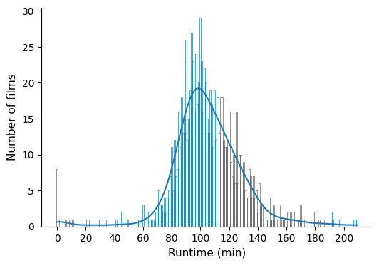
We see that there are about 8 movies with a duration of 0 minutes. This is because the value of this field was not filled in the TMDB record, so we discard them before calculating the average duration value of the films.

Show code cell source Hide code cell source

# Remove records with runtime 0
films_t = films.loc[films['tmdb_runtime'] > 0, :]

# Print mean value
print(f"Mean duration is --> {films_t['tmdb_runtime'].mean():.0f} minutes")

Mean duration is --> 106 minutes

Therefore, the average duration of a feature film is approximately one hour and three quarters, which matches the idea I had.

Out of curiosity, I extract the ten longest movies from those I have seen.

Show code cell source Hide code cell source

# Define list with columns to show
show_cols = ['director', 'year', 'tmdb_title', 'tmdb_runtime']

# Print ten most lengthy movies
films_t.loc[:, show_cols]\
            .sort_values(by=['tmdb_runtime'], ascending=False).head(10)

	director	year	tmdb_title	tmdb_runtime
801	Martin Scorsese	2019	The Irishman	209
655	Martin Scorsese	2005	No Direction Home: Bob Dylan	208
139	Akira Kurosawa	1954	Seven Samurai	207
511	Nuri Bilge Ceylan	2014	Winter Sleep	196
299	Robert B. Weide	2012	Woody Allen: A Documentary	192
607	Richard Attenborough	1982	Gandhi	191
180	Marcel Carné	1945	Children of Paradise	191
30	Luchino Visconti	1963	The Leopard	186
259	Andrei Tarkovsky	1966	Andrei Rublev	183
0	David Lynch	2006	Inland Empire	180

Next, I plot the movies based on their duration, distinguishing between documentaries and fiction films on the graph. I include the yearly mean value on the graph as well.

Show code cell source Hide code cell source

# Plot
fig, ax = plt.subplots(figsize=(7, 7))


sns.scatterplot(x="year", y="tmdb_runtime", data=films_t, ax=ax, alpha=0.5,
                hue="tmdb_genre", hue_order=['Film', 'Documentary'])

films_t.pivot_table(index='year', values='tmdb_runtime', aggfunc='mean').plot(ax=ax, color='black')

ax.set_xlabel("", fontsize=11)
ax.set_ylabel("Runtime", fontsize=11)
ax.legend(bbox_to_anchor=(1.0, 0.5), loc='center left', fontsize=10,
          labels=['', 'Film', 'Documentary', 'Mean value'])
sns.despine()

plt.show()

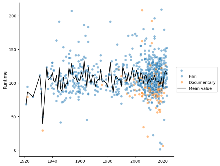
In the graph, it can be observed that the majority of the movies I have seen are from recent years. Regarding their duration, it does not seem to have increased. However, I am going to focus the graph on the last 20 years, from 2004 to 2024, and I am going to exclude the documentaries to see if there is an upward trend in duration or if such a trend does not exist.

Show code cell source Hide code cell source

# Define cut-off year
y = 2004

# Get only films in the last "y" years and not documentaries
films_ty = films_t.loc[(films_t['year'] >= y) & (films_t['tmdb_genre'] == 'Film'), :]

# Plot
fig, ax = plt.subplots(figsize=(7, 7))

sns.scatterplot(x="year", y="tmdb_runtime", data=films_ty, ax=ax, alpha=0.5)

films_ty.pivot_table(index='year', values='tmdb_runtime', aggfunc='mean').plot(ax=ax, color='black')

ax.set_xlabel("", fontsize=11)
ax.set_ylabel("Movie duration", fontsize=11)
ax.legend(bbox_to_anchor=(1.0, 0.5), loc='center left', fontsize=10, labels=['Film', 'Mean value'])
ax.set_xticks(range(2004, 2024, 2), labels=list(np.arange(2004, 2024, 2)))
sns.despine()

plt.show()

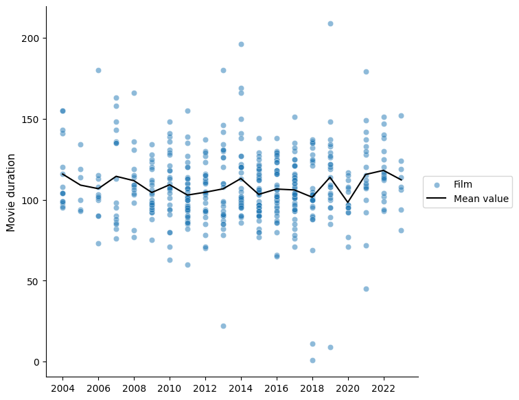
I would say there hasn’t been a significant change in the duration of the movies, at least in the ones I’ve seen, so the notion that movies are getting longer must be just my impression that doesn’t align with reality.

Rating analysis

To ensure consistency in the movie ratings, I will only consider movies that have received a minimum of, for example, 100 ratings.

Show code cell source Hide code cell source

# Minimum number of votings to consider movie rating valid
v = 100

# Get films with at least 100 votes
films_v = films.loc[films['tmdb_vote_cnt'] >= v, :]

# Print how many of them there are
print(f"{len(films_v)} out of the {len(films)} movies have more than {v} votes in TMDb")

648 out of the 927 movies have more than 100 votes in TMDb

These are the 10 movies that have received the most number of ratings:

Show code cell source Hide code cell source

# Define list of columns to show
show_cols = ['director', 'year', 'tmdb_title', 'tmdb_vote_cnt', 'tmdb_vote_avg']

# Print most voted movies
films_v.loc[:, show_cols]\
            .sort_values(by=['tmdb_vote_cnt'], ascending=False).head(10)

	director	year	tmdb_title	tmdb_vote_cnt	tmdb_vote_avg
468	Christopher Nolan	2014	Interstellar	33563	8.4
792	Todd Phillips	2019	Joker	24056	8.2
618	Pete Docter	2015	Inside Out	19984	7.9
818	Joon-ho Bong	2019	Parasite	17057	8.5
627	Denis Villeneuve	2016	Arrival	16927	7.6
919	Olivier Nakache	2011	The Intouchables	16499	8.3
539	Morten Tyldum	2014	The Imitation Game	16309	8.0
580	Damien Chazelle	2016	La La Land	15977	7.9
650	Christopher Nolan	2017	Dunkirk	15792	7.5
577	Hayao Miyazaki	2001	Spirited Away	15490	8.5

And these are the ones that have received the highest ratings:

Show code cell source Hide code cell source

# Print most rated movies
films_v.loc[:, show_cols]\
            .sort_values(by=['tmdb_vote_avg'], ascending=False).head(10)

	director	year	tmdb_title	tmdb_vote_cnt	tmdb_vote_avg
34	Sergio Leone	1966	The Good, the Bad and the Ugly	8062	8.5
818	Joon-ho Bong	2019	Parasite	17057	8.5
442	Giuseppe Tornatore	1988	Cinema Paradiso	4108	8.5
816	Isao Takahata	2003	Grave of the Fireflies	5087	8.5
139	Akira Kurosawa	1954	Seven Samurai	3391	8.5
577	Hayao Miyazaki	2001	Spirited Away	15490	8.5
489	Damien Chazelle	2014	Whiplash	14324	8.4
426	Milos Forman	1975	One Flew Over the Cuckoo's Nest	9921	8.4
409	Carlos Sorin	2008	Rear Window	6118	8.4
230	Fernando Meirelles	2002	City of God	6920	8.4

For a clearer visual reference, I place these movies into three different groups corresponding to my personal ratings of them.

Show code cell source Hide code cell source

# Plot
fig, ax = plt.subplots(figsize=(7, 7))

warnings.filterwarnings('ignore') # swarmplot does not fit, but ignore warning
sns.swarmplot(ax=ax, x="stars", y="tmdb_vote_avg", data=films_v, alpha=0.75,
              order=['untagged', 'liked', 'loved'],
              hue="tmdb_genre", hue_order=['Film', 'Documentary'])

sns.boxplot(ax=ax, x="stars", y="tmdb_vote_avg", data=films_v,
              boxprops=dict(linewidth=1, facecolor='white', edgecolor='grey', alpha=1),
                whiskerprops=dict(linewidth=1, color='grey', alpha=1),
                medianprops=dict(linewidth=1, color="grey", alpha=1),
                capprops=dict(linewidth=1, color='grey', alpha=1)
)

ax.set_xlabel("", fontsize=11)
ax.set_ylabel("Rating in TMDb", fontsize=11)
ax.set_xticks(range(3), labels=['I did not tag them',
                                'I liked them', 'I loved them'])
ax.legend(bbox_to_anchor=(1.0, 0.5), loc='center left', fontsize=10)
sns.despine()

plt.show()

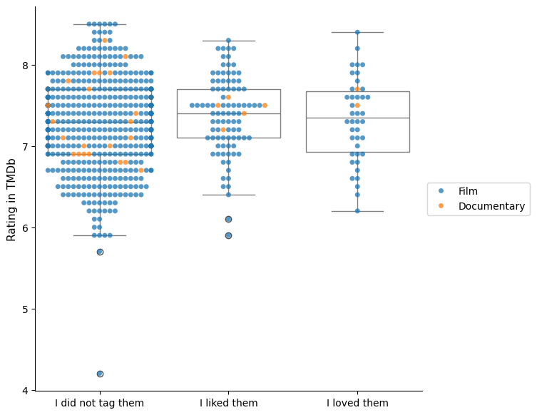
In the graph, I see that among the ones I loved, there are a couple of movies that also enjoyed much public favor. Which ones are they?

Show code cell source Hide code cell source

# Append my valoration to print
show_cols.append('stars')

# Show maximum rating movies among loved ones
films_v.loc[films_v['stars'] == 'loved', show_cols]\
            .sort_values(by='tmdb_vote_avg', ascending=False).head(2)

	director	year	tmdb_title	tmdb_vote_cnt	tmdb_vote_avg	stars
426	Milos Forman	1975	One Flew Over the Cuckoo's Nest	9921	8.4	loved
193	Billy Wilder	1960	The Apartment	2103	8.2	loved

Oh, definitely!

Which is that film that I loved, but got a lower rating in TMDB?

Show code cell source Hide code cell source

# Show the movie with less rating among the loved ones
films_v.loc[films_v['stars'] == 'loved', show_cols]\
            .sort_values(by='tmdb_vote_avg').head(1)

	director	year	tmdb_title	tmdb_vote_cnt	tmdb_vote_avg	stars
658	Manuel Martín Cuenca	2017	The Motive	257	6.2	loved

And what about the movies that I didn’t label because they didn’t particularly strike me (or I forgot to label them), yet they have high ratings? I list the six that appear at the top of the graph in the untagged group.

Show code cell source Hide code cell source

# Show maximum rating movie among untagged ones
films_v.loc[films_v['stars'] == 'untagged', show_cols]\
            .sort_values(by='tmdb_vote_avg', ascending=False).head(6)

	director	year	tmdb_title	tmdb_vote_cnt	tmdb_vote_avg	stars
818	Joon-ho Bong	2019	Parasite	17057	8.5	untagged
139	Akira Kurosawa	1954	Seven Samurai	3391	8.5	untagged
816	Isao Takahata	2003	Grave of the Fireflies	5087	8.5	untagged
577	Hayao Miyazaki	2001	Spirited Away	15490	8.5	untagged
34	Sergio Leone	1966	The Good, the Bad and the Ugly	8062	8.5	untagged
442	Giuseppe Tornatore	1988	Cinema Paradiso	4108	8.5	untagged

I definitely should have uprated Parasite! (But by no means Cinema Paradiso).

And what’s that movie that’s so low in the ratings?

Show code cell source Hide code cell source

# Show that outlier among untagged ones
films_v.loc[films_v['stars'] == 'untagged', show_cols]\
            .sort_values(by='tmdb_vote_avg').head(1)

	director	year	tmdb_title	tmdb_vote_cnt	tmdb_vote_avg	stars
142	Ed. Wood	1959	Plan 9 from Outer Space	509	4.2	untagged

It’s the famous Ed Wood movie, considered to be the worst in the history of cinema!

Original languages

Once we’re in the thick of it, I found it interesting to consider the original language of the movies I’ve watched over these years. Perhaps this information would tell me something about the type of cinema I prefer.

Show code cell source Hide code cell source

# Define number of languages
n = 10

# Get the n most frequent languages
films_nlang = films.value_counts('tmdb_lang').head(n)

# Convert their language codes into full names
films_nlang = films_nlang.reset_index()
films_nlang['tmdb_lang'] = [Lang(s).name for s in films_nlang['tmdb_lang']]
films_nlang = films_nlang.set_index('tmdb_lang')

# Plot
fig, ax = plt.subplots(figsize=(6, 4))

films_nlang.plot(ax=ax, kind="barh")

ax.grid(axis="x")
ax.set_axisbelow(True)
ax.set_title("Most common original languages", size=11)
ax.set_xlabel("number of movies", fontsize=11)
ax.set_ylabel("", fontsize=11)
ax.legend().set_visible(False)
ax.invert_yaxis()
sns.despine()

plt.show()

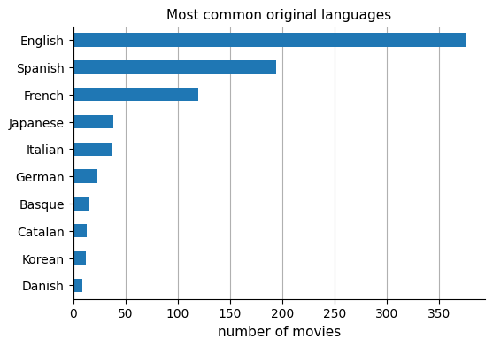
The top three main languages were as expected, and so were the following ones. As Korean and Danish appear on this list, it confirms the special interest I have in the cinema of these countries.

Conclusion

This little project allowed me to analyze the personal movie record I’ve been updating for some years. I found it interesting to have the option to automatically add further data of each movie from TMDB, as it saves me the trouble of doing it manually, and my table has indeed become more comprehensive.

Regarding the questions I had in mind, it seems that the duration of the films does not tend to increase, at least not significantly, after an analysis that has been purely visual.

As for the community ratings and whether they are in line with my tastes, well, it’s a bit of everything. However, one thing that is clear is that TMDB ratings don’t help much in identifying good movies since the vast majority fall between 6 and 8 points. However, they do help in recognizing big hits based on the number of ratings.