Employee Network Analysis

Employee Network Analysis#

A DataCamp challenge Mar, 2024

Network analysis

The project#

You work in the analytics department of a multinational company, and the head of HR wants your help mapping out the company’s employee network using message data.

They plan to use the network map to understand interdepartmental dynamics better and explore how the company shares information. The ultimate goal of this project is to think of ways to improve collaboration throughout the company.

Create a report that covers the following:

Which departments are the most/least active?
Which employee has the most connections?
Identify the most influential departments and employees.
Using the network analysis, in which departments would you recommend the HR team focus to boost collaboration?

The data#

The company has six months of information on inter-employee communication. For privacy reasons, only sender, receiver, and message length information are available (source).

Messages has information on the sender, receiver, and time.

“sender” - represents the employee id of the employee sending the message.
“receiver” - represents the employee id of the employee receiving the message.
“timestamp” - the date of the message.
“message_length” - the length in words of the message.

Employees has information on each employee.

“id” - represents the employee id of the employee.
“department” - is the department within the company.
“location” - is the country where the employee lives.
“age” - is the age of the employee.

Acknowledgments: Pietro Panzarasa, Tore Opsahl, and Kathleen M. Carley. “Patterns and dynamics of users’ behavior and interaction: Network analysis of an online community.” Journal of the American Society for Information Science and Technology 60.5 (2009): 911-932.

	sender	receiver	timestamp	message_length
0	79	48	2021-06-02 05:41:34	88
1	79	63	2021-06-02 05:42:15	72
2	79	58	2021-06-02 05:44:24	86
3	79	70	2021-06-02 05:49:07	26
4	79	109	2021-06-02 19:51:47	73
...	...	...	...	...
3507	469	1629	2021-11-24 05:04:57	75
3508	1487	1543	2021-11-26 00:39:43	25
3509	144	1713	2021-11-28 18:30:47	51
3510	1879	1520	2021-11-29 07:27:52	58
3511	1879	1543	2021-11-29 07:37:49	56

3512 rows × 4 columns

	id	department	location	age
0	3	Operations	US	33
1	6	Sales	UK	50
2	8	IT	Brasil	54
3	9	Admin	UK	32
4	12	Operations	Brasil	51
...	...	...	...	...
659	1830	Admin	UK	42
660	1839	Admin	France	28
661	1879	Engineering	US	40
662	1881	Sales	Germany	57
663	1890	Admin	US	39

664 rows × 4 columns

Company#

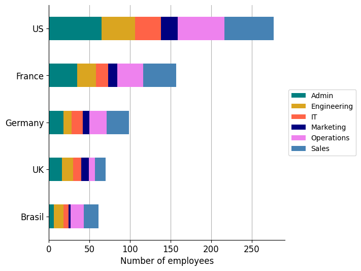
The following graph shows the distribution, by location and by departments, of the 664 employees of the company.

../_images/4c291f8fdd2a0db42a3a97b4d554187f14a26aa7044baaeecedf2cd2c38bd64f.png

Messages#

Between departments#

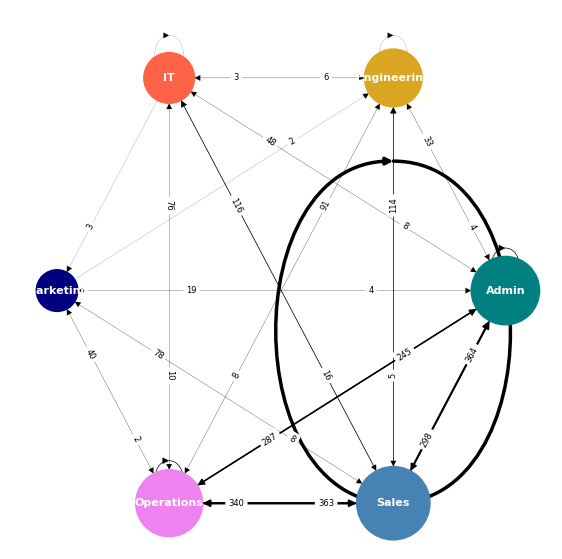
These are the number of messages sent between departments. The size of the nodes represents the number of employees that each department has.

Show code cell source Hide code cell source

# Merge messages-employees dataframes on sender ids
senders = messages.merge(employees, how="left", left_on="sender", right_on="id").drop(
    "id", axis=1
)

# Rename columns
senders = senders.rename(
    columns={"department": "s_dep", "location": "s_loc", "age": "s_age"}
)

# Merge messages-employees dataframes on receiver ids
senders_receivers = senders.merge(
    employees, how="left", left_on="receiver", right_on="id"
).drop("id", axis=1)

# Rename columns
senders_receivers = senders_receivers.rename(
    columns={"department": "r_dep", "location": "r_loc", "age": "r_age"}
)

# senders_receivers.head()

# Pivot table on sender-receiver departments to count messages sent
dep_table = senders_receivers.pivot_table(
    index="s_dep", columns="r_dep", values="sender", aggfunc="count"
)

# Create a directional graph
D = nx.DiGraph()

# Add nodes: the set of departments
D.add_nodes_from(dep_table.index)

# Add edges
dep_edges = []
dep_msgs = []
for i in range(len(dep_table.index)):
    for j in range(len(dep_table.columns)):
        msgs = dep_table.iloc[i, j]
        if msgs > 0:
            dep_edges.append((dep_table.index[i], dep_table.columns[j]))
            dep_msgs.append(msgs)  # Store them to add metadata later

D.add_edges_from(dep_edges)

# Add metadata (number of messages) for each edge
for edge, message in zip(D.edges, dep_msgs):
    D.edges[edge]["messages"] = message.astype(int)

# D.edges(data=True) # Print edges with metadata

# Node colors
color_key = {department: color for department, color in zip(dep_table.index, palette)}
node_colors = [color_key[dept] for dept in D.nodes]

# Node size according to number of employees by department
department_employees = employees.groupby("department")["id"].count()
scale = 900  # Just to match desired size in the plot
dep_node_sizes = scale * department_employees / min(department_employees)

# Linewidth of the edges according to number of messages
dep_msgs_df = pd.DataFrame(dep_msgs, columns=["msgs"])
bins = [0, 100, 200, 300, 400, 500, 1000]
widths = [0.1, 0.5, 1.0, 1.5, 2.0, 2.5]
dep_msgs_df["linewidth"] = pd.cut(dep_msgs_df["msgs"], bins, labels=widths)
dep_msgs_df["dep_edges"] = dep_edges
linewidth_edges = dep_msgs_df.groupby("linewidth", observed=False)["dep_edges"].apply(
    list
)

# Layout of the graph
pos = nx.circular_layout(D)

# Plot
fig, ax = plt.subplots(figsize=(7, 7))

nx.draw_networkx_nodes(D, pos, ax=ax, node_size=dep_node_sizes, node_color=node_colors)
nx.draw_networkx_labels(
    D, pos, ax=ax, font_size=8, font_weight="bold", font_color="white"
)

for linewidth, edgelist in linewidth_edges.items():
    nx.draw_networkx_edges(
        D,
        pos,
        ax=ax,
        arrows=True,
        edgelist=edgelist,
        width=linewidth,
        node_size=list(dep_node_sizes),
    )

nx.draw_networkx_edge_labels(
    D,
    pos,
    ax=ax,
    edge_labels=nx.get_edge_attributes(D, "messages"),
    label_pos=0.3,
    font_size=6,
)

ax.axis("off")
plt.show()

../_images/f9c52716dca08acc1d9c8a66642c4c33db7c1e6139b43010c1502549563adb3e.png

../_images/ee866d12a8592a829c424250e6aa69d6dd2a0119dd4de72a8f54b4004e999d4f.png

In the following graph, the size of the nodes represents the number of messages sent by each employee in that department, which is the number displayed in the node. The thickness of the connections is proportional to that quantity.

Show code cell source Hide code cell source

# Create a directional graph
D_rel = nx.DiGraph()

# Add nodes: the set of departments
D_rel.add_nodes_from(dep_table_rel.index)

# Add edges
dep_edges = []
dep_msgs = []
for i in range(len(dep_table_rel.index)):
    for j in range(len(dep_table_rel.columns)):
        msgs = dep_table_rel.iloc[i, j]
        if msgs > 0:
            dep_edges.append((dep_table_rel.index[i], dep_table_rel.columns[j]))
            dep_msgs.append(msgs)  # Store them to add metadata later

D_rel.add_edges_from(dep_edges)

# Add metadata (number of messages) for each edge
for edge, message in zip(D_rel.edges, dep_msgs):
    D_rel.edges[edge]["messages"] = message.astype(int)

# D.edges(data=True) # Print edges with metadata

# Node colors
color_key = {department: color for department, color in zip(dep_table.index, palette)}
node_colors = [color_key[dept] for dept in D_rel.nodes]

# Node size according to number of messages sent by department
sent_per_employee = round(dep_table_rel.sum(axis=1), 1)
scale = 300  # Just to match desired size in the plot
dep_node_sizes = scale * sent_per_employee

# Labels
labels = {
    n: str(n) + "\n" + str(sent) for n, sent in zip(D_rel.nodes(), sent_per_employee)
}

# Linewidth of the edges according to number of messages
dep_msgs_df = pd.DataFrame(dep_msgs, columns=["msgs"])
bins = [0, 1, 2, 3, 4, 5, 6, 7, 8, 9, 10]
widths = [0.1, 1.5, 2.0, 3.5, 4.0, 5.5, 6.0, 7.5, 8.0, 9.5]
dep_msgs_df["linewidth"] = pd.cut(dep_msgs_df["msgs"], bins, labels=widths)
dep_msgs_df["dep_edges"] = dep_edges
linewidth_edges = dep_msgs_df.groupby("linewidth", observed=False)["dep_edges"].apply(
    list
)

# Layout of the graph
pos = nx.spiral_layout(D_rel)

# Plot
fig, ax = plt.subplots(figsize=(6, 6))

nx.draw_networkx_nodes(
    D_rel, pos, ax=ax, node_size=dep_node_sizes, node_color=node_colors
)
nx.draw_networkx_labels(
    D_rel,
    pos,
    ax=ax,
    font_size=8,
    font_weight="bold",
    font_color="white",
    labels=labels,
)

for linewidth, edgelist in linewidth_edges.items():
    nx.draw_networkx_edges(
        D_rel,
        pos,
        ax=ax,
        edgelist=edgelist,
        width=linewidth,
        node_size=list(dep_node_sizes),
    )

ax.legend(legend_h, legend_l, bbox_to_anchor=(1.0, 0.5), loc="center left", fontsize=10)

ax.axis("off")
plt.show()

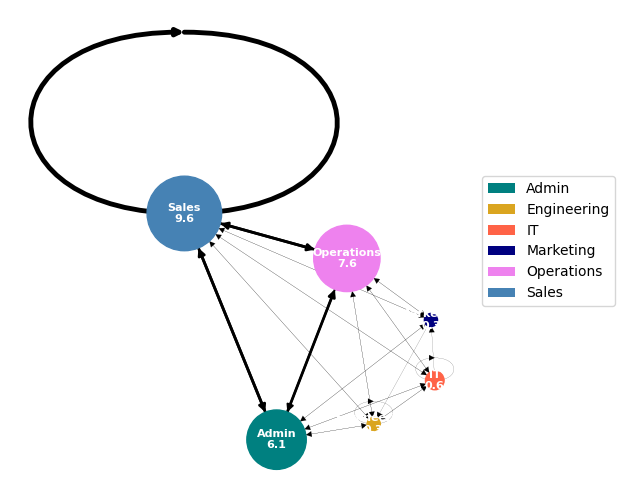
../_images/6fceac0532662ef9e958361e54679ef0d105190a2d453433047197d91d765086.png

The graph clearly shows that the majority of the traffic is generated by the triangle formed by the Sales, Admin, and Operations. Employees working in these departments send an average of more than six messages, while others do not reach even one message per employee.

The metric called Degree Centrality is a measure of the number of neighbors a node has, divided by the total number it could possibly have.

Degree centrality:

Admin --> 1.0
Operations --> 1.0
Sales --> 1.0
Engineering --> 0.9
IT --> 0.9
Marketing --> 0.7

These data indicate what we had already seen in the previous tables: while Admin Operations and Sales send to and receive from all departments, the rest lack some form of communication. Engineering is not sending to Marketing and IT is not receiving from Marketing. Marketing are not sending to IT and they do not send messages to themselves.

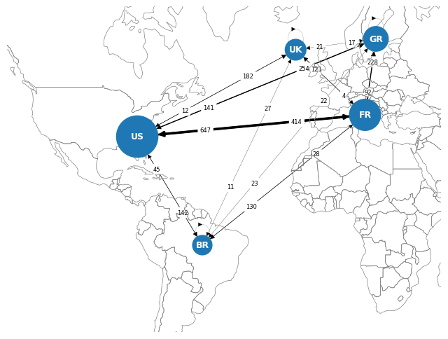
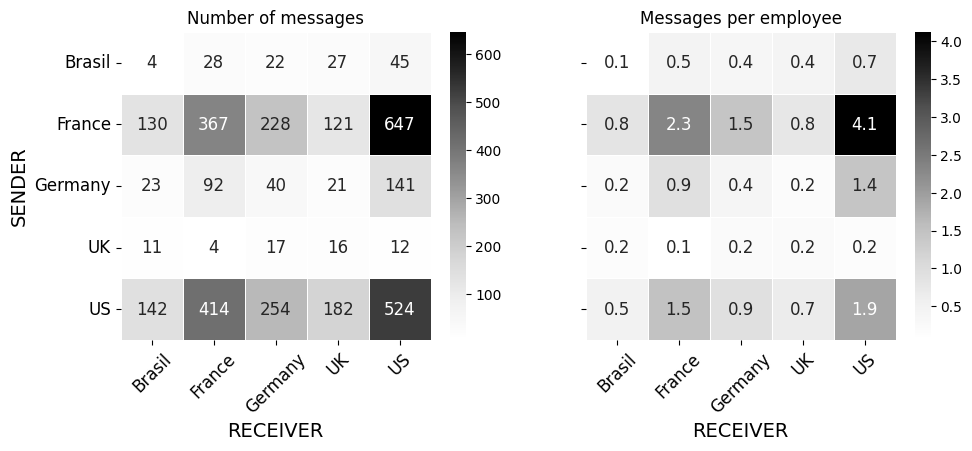
Between locations#

These are the number of messages sent between locations. The size of the nodes represents the number of employees that each location has.

Show code cell source Hide code cell source

# Pivot table on sender-receiver locations to count messages sent
loc_table = senders_receivers.pivot_table(
    index="s_loc", columns="r_loc", values="sender", aggfunc="count"
)

# Create a directional graph
C = nx.DiGraph()

# Add nodes: the set of locations
C.add_nodes_from(loc_table.index)

# Add edges
loc_edges = []
loc_msgs = []
for i in range(len(loc_table.index)):
    for j in range(len(loc_table.columns)):
        msgs = loc_table.iloc[i, j]
        if msgs > 0:
            loc_edges.append((loc_table.index[i], loc_table.columns[j]))
            loc_msgs.append(msgs)  # Store them to add metadata later

C.add_edges_from(loc_edges)

# Add metadata (number of messages) for each edge
for edge, message in zip(C.edges, loc_msgs):
    C.edges[edge]["messages"] = message.astype(int)

# Node size according to number of employees by location
location_employees = employees.groupby("location")["id"].count()
scale = 400  # Just to match desired size in the plot
loc_node_sizes = scale * location_employees / min(location_employees)

# Linewidth of the edges according to number of messages
loc_msgs_df = pd.DataFrame(loc_msgs, columns=["msgs"])
bins = [0, 100, 200, 300, 400, 500, 1000]
widths = [0.1, 0.5, 1.0, 1.5, 2.0, 2.5]
loc_msgs_df["linewidth"] = pd.cut(loc_msgs_df["msgs"], bins, labels=widths)
loc_msgs_df["loc_edges"] = loc_edges
linewidth_edges = loc_msgs_df.groupby("linewidth", observed=False)["loc_edges"].apply(
    list
)

# Layout of the graph
# Adjust manually country positions for readibility
location_key = {
    "Brasil": (-6000000, -1000000),
    # "Brasil": (-4810350.913, -2620812.957),
    "France": (1500000, 5000000),
    # "France": (261933.923, 6250816.842),
    "Germany": (2000000, 8500000),
    # "Germany": (1491636.961, 6895388.529),
    "UK": (-1700000, 8000000),
    # "UK": (-13210.028, 6710566.113),
    "US": (-9000000, 4000000),
    # "US": (-8237165.598, 4971358.429),
}
pos = {n: location_key[n] for n in C.nodes()}

# Labels
label_key = {"Brasil": "BR", "France": "FR", "Germany": "GR", "UK": "UK", "US": "US"}
labels = {n: label_key[n] for n in C.nodes()}

# Prepare world map background from GeoPandas in projection 3857
# naturalearth_lowres = gpd.read_file(gpd.datasets.get_path("naturalearth_lowres")) # <- deprecated
naturalearth_lowres = gpd.read_file("map/ne_110m_admin_0_countries.shp")
naturalearth_lowres_3857 = naturalearth_lowres.copy()
naturalearth_lowres_3857.geometry = naturalearth_lowres_3857.geometry.to_crs(epsg=3857)

# Plot
fig, ax = plt.subplots(figsize=(8, 8))

naturalearth_lowres_3857.boundary.plot(ax=ax, edgecolor="grey", linewidth=0.5)
ax.set_xlim(-1.5e7, 0.5e7)
ax.set_ylim(-0.5e7, 1e7)

nx.draw_networkx_nodes(C, pos, ax=ax, node_size=loc_node_sizes)
nx.draw_networkx_labels(
    C, pos, ax=ax, font_size=9, font_weight="bold", font_color="white", labels=labels
)

for linewidth, edgelist in linewidth_edges.items():
    nx.draw_networkx_edges(
        C,
        pos,
        ax=ax,
        arrows=True,
        edgelist=edgelist,
        width=linewidth,
        node_size=list(loc_node_sizes),
    )

nx.draw_networkx_edge_labels(
    C,
    pos,
    ax=ax,
    edge_labels=nx.get_edge_attributes(C, "messages"),
    label_pos=0.3,
    font_size=6,
    rotate=False,
)

ax.axis("off")
plt.show()

../_images/d37079cca813feb2bc48319eb337b38d7484c812e81c3e511bad18eb809782b8.png

../_images/8ee04439852ee5fdc3986bf7f3aa3b68c83af1b989146afee512ec2006d563cb.png

In the following graph, the size of the nodes represents the number of messages sent by employee in each location, which is the number displayed in the node. The thickness of the connections is proportional to that quantity.

Show code cell source Hide code cell source

# Create a directional graph
C_rel = nx.DiGraph()

# Add nodes: the set of departments
C_rel.add_nodes_from(loc_table_rel.index)

# Add edges
dep_edges = []
dep_msgs = []
for i in range(len(loc_table_rel.index)):
    for j in range(len(loc_table_rel.columns)):
        msgs = loc_table_rel.iloc[i, j]
        if msgs > 0:
            dep_edges.append((loc_table_rel.index[i], loc_table_rel.columns[j]))
            dep_msgs.append(msgs)  # Store them to add metadata later

C_rel.add_edges_from(dep_edges)

# Add metadata (number of messages) for each edge
for edge, message in zip(C_rel.edges, dep_msgs):
    C_rel.edges[edge]["messages"] = message.astype(int)


# Node size according to number of messages sent by department
sent_per_employee = round(loc_table_rel.sum(axis=1), 1)
scale = 300  # Just to match desired size in the plot
dep_node_sizes = scale * sent_per_employee

# Labels
label_key = {"Brasil": "BR", "France": "FR", "Germany": "GR", "UK": "UK", "US": "US"}
labels = {
    n: label_key[n] + "\n" + str(sent)
    for n, sent in zip(C_rel.nodes(), sent_per_employee)
}

# Linewidth of the edges according to number of messages
dep_msgs_df = pd.DataFrame(dep_msgs, columns=["msgs"])
bins = [0, 1, 2, 3, 4, 5, 6, 7, 8, 9, 10]
widths = [0.1, 1.5, 2.0, 3.5, 4.0, 5.5, 6.0, 7.5, 8.0, 9.5]
dep_msgs_df["linewidth"] = pd.cut(dep_msgs_df["msgs"], bins, labels=widths)
dep_msgs_df["dep_edges"] = dep_edges
linewidth_edges = dep_msgs_df.groupby("linewidth", observed=False)["dep_edges"].apply(
    list
)

# Layout of the graph
pos = nx.shell_layout(C_rel)

# Plot
fig, ax = plt.subplots(figsize=(6, 6))

nx.draw_networkx_nodes(C_rel, pos, ax=ax, node_size=dep_node_sizes)
nx.draw_networkx_labels(
    C_rel,
    pos,
    ax=ax,
    font_size=8,
    font_weight="bold",
    font_color="white",
    labels=labels,
)

for linewidth, edgelist in linewidth_edges.items():
    nx.draw_networkx_edges(
        C_rel,
        pos,
        ax=ax,
        edgelist=edgelist,
        width=linewidth,
        node_size=list(dep_node_sizes),
    )

ax.axis("off")
plt.show()

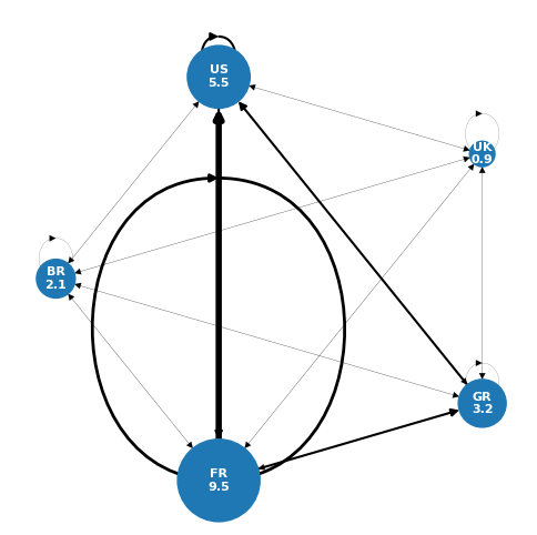
../_images/ab293e505a45b796986543bc425239f523ab5118f157264e41a3224138e968f4.png

The predominance of France is clearly evident, with nearly 10 messages per employee, most of them directed towards the US, which comes second. Following are Germany, Brazil, and lastly the UK, which doesn’t even reach one email sent per employee.

Nevertheless, all countries have communicated with each other according to the values of Degree Centrality.

Degree centrality:

Brasil --> 1.0
France --> 1.0
Germany --> 1.0
UK --> 1.0
US --> 1.0

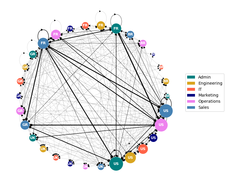
Departments in locations#

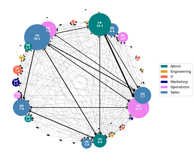
Let’s consider messages sent by each department in each location. The size of the nodes represents the number of employees that each department has at that particular location.

Show code cell source Hide code cell source

# Pivot table on sender-receiver departments and locations to count messages sent
msg_table = senders_receivers.pivot_table(
    index=["s_loc", "s_dep"],
    columns=["r_loc", "r_dep"],
    values="sender",
    aggfunc="count",
)

# Create a directional graph
DC = nx.DiGraph()

# Add nodes: the set of departments
DC.add_nodes_from(msg_table.columns)

# Add edges
deploc_edges = []
deploc_msgs = []
for i in range(len(msg_table.index)):
    for j in range(len(msg_table.columns)):
        msgs = msg_table.iloc[i, j]
        if msgs > 0:
            deploc_edges.append((msg_table.index[i], msg_table.columns[j]))
            deploc_msgs.append(msgs)

DC.add_edges_from(deploc_edges)

# Add metadata (number of messages) for each edge
for edge, message in zip(DC.edges, deploc_msgs):
    DC.edges[edge]["messages"] = message.astype(int)

# Plotting to a polygon background

node_color = []
for n in range(len(DC.nodes())):
    node_color.append(color_key[list(DC.nodes())[n][1]])

# Node size according to number of employees by department
location_department_employees = employees.groupby(["location", "department"])[
    "id"
].count()
scale = 50
node_sizes = scale * location_department_employees / min(location_department_employees)


# Linewidth of the edges according to number of messages
deploc_msgs_df = pd.DataFrame(deploc_msgs, columns=["msgs"])
bins = [0, 20, 40, 60, 80, 100, 1000]
widths = [0.1, 0.5, 1.0, 1.5, 2.0, 2.5]
deploc_msgs_df["linewidth"] = pd.cut(deploc_msgs_df["msgs"], bins, labels=widths)
deploc_msgs_df["deploc_edges"] = deploc_edges
linewidth_edges = deploc_msgs_df.groupby("linewidth", observed=False)[
    "deploc_edges"
].apply(list)


pos = nx.circular_layout(DC)

label_key = {"Brasil": "BR", "France": "FR", "Germany": "GR", "UK": "UK", "US": "US"}
labels = {
    n: label_key[list(DC.nodes())[i][0]]
    for n, i in zip(DC.nodes(), range(len(list(DC.nodes()))))
}


# Plot
fig, ax = plt.subplots(figsize=(8, 8))

nx.draw_networkx_nodes(DC, pos, ax=ax, node_size=node_sizes, node_color=node_color)
nx.draw_networkx_labels(
    DC, pos, ax=ax, font_size=9, font_weight="bold", font_color="white", labels=labels
)

for linewidth, edgelist in linewidth_edges.items():
    nx.draw_networkx_edges(
        DC,
        pos,
        ax=ax,
        arrows=True,
        edgelist=edgelist,
        width=linewidth,
        node_size=list(node_sizes),
    )

ax.legend(legend_h, legend_l, bbox_to_anchor=(1.0, 0.5), loc="center left", fontsize=10)

ax.axis("off")
plt.show()

../_images/2a60de3b194fd599c4b162277522de693e1d065e0632ea72d0bffcb31cba16be.png

../_images/e340954391e446ab34245906ef962ee5791926fd7f8f7b01d8b9031dc17ec6f1.png

In the following graph, the size of the nodes represents the number of messages sent by employee in each department and location, which is the number displayed in the node. The thickness of the connections is proportional to that quantity.

Show code cell source Hide code cell source

# Create a directional graph
DC_rel = nx.DiGraph()

# Add nodes: the set of departments
DC_rel.add_nodes_from(msg_table_rel.index)

# Add edges
dep_edges = []
dep_msgs = []
for i in range(len(msg_table_rel.index)):
    for j in range(len(msg_table_rel.columns)):
        msgs = msg_table_rel.iloc[i, j]
        if msgs > 0:
            dep_edges.append((msg_table_rel.index[i], msg_table_rel.columns[j]))
            dep_msgs.append(msgs)  # Store them to add metadata later

DC_rel.add_edges_from(dep_edges)

# Add metadata (number of messages) for each edge
for edge, message in zip(DC_rel.edges, dep_msgs):
    DC_rel.edges[edge]["messages"] = message.astype(int)

# Node colors
color_key = {department: color for department, color in zip(dep_table.index, palette)}
node_colors = []
for n in DC_rel.nodes:
    node_colors.append(color_key[n[1]])
    # node_colors.append(color_key[list(DC_rel.nodes())[n][1]])

# Node size according to number of messages sent by department
sent_per_employee = round(msg_table_rel.sum(axis=1), 1)
scale = 300  # Just to match desired size in the plot
dep_node_sizes = scale * sent_per_employee

# Labels
label_key = {"Brasil": "BR", "France": "FR", "Germany": "GR", "UK": "UK", "US": "US"}
labels = {
    n: label_key[n[0]] + "\n" + str(sent)
    for n, sent in zip(DC_rel.nodes(), sent_per_employee)
}


# Linewidth of the edges according to number of messages
dep_msgs_df = pd.DataFrame(dep_msgs, columns=["msgs"])
bins = [0, 1, 2, 3, 4, 5, 6, 7, 8, 9, 10]
widths = [0.1, 1.5, 2.0, 3.5, 4.0, 5.5, 6.0, 7.5, 8.0, 9.5]
dep_msgs_df["linewidth"] = pd.cut(dep_msgs_df["msgs"], bins, labels=widths)
dep_msgs_df["dep_edges"] = dep_edges
linewidth_edges = dep_msgs_df.groupby("linewidth", observed=False)["dep_edges"].apply(
    list
)

# Layout of the graph
pos = nx.circular_layout(DC_rel)

# Plot
fig, ax = plt.subplots(figsize=(8, 8))

nx.draw_networkx_nodes(
    DC_rel, pos, ax=ax, node_size=dep_node_sizes, node_color=node_colors
)
nx.draw_networkx_labels(
    DC_rel,
    pos,
    ax=ax,
    font_size=8,
    font_weight="bold",
    font_color="white",
    labels=labels,
)

for linewidth, edgelist in linewidth_edges.items():
    nx.draw_networkx_edges(
        DC_rel,
        pos,
        ax=ax,
        edgelist=edgelist,
        width=linewidth,
        node_size=list(dep_node_sizes),
    )

ax.legend(legend_h, legend_l, bbox_to_anchor=(1.0, 0.5), loc="center left", fontsize=10)

ax.axis("off")
plt.show()

../_images/2e30aec5ae698a0867c792fe1709dd1e76e299d8a2af1f01e445ccddfb104d94.png

Next, I will represent in a comparative graph the values of the following parameters:

Degree Centrality: already mentioned, this is the number of neighbors a node has, divided by the total number it could possibly have.
Betweennness Centrality: is defined as the number of shortest paths in a graph that pass through a node divided by the number of shortest paths that exist between every pair of nodes in a graph. It captures bottleneck nodes in a graph, rather than highly connected nodes.

../_images/bdffb037ee38ca99a1a39f7ba48aaecd3726b37b7d5454d157ba456c05c37ef3.png

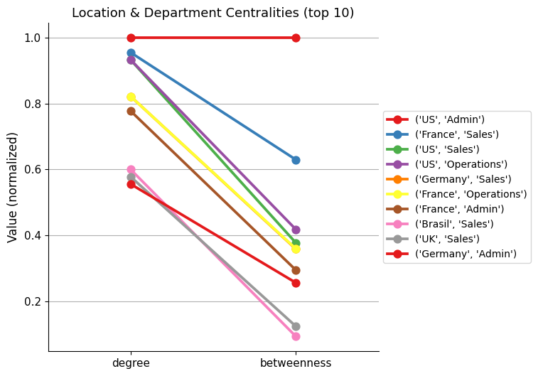
From this chart we learn that US Admin, despite not being the department that sends the most messages per employee, does have a prevalent position because it has the most connections in the network and serves as the main connecting point for the traffic in the network. So US Admin is the most influential node and the most critical one.

Employee network#

First of all, I’m going to take a look at the number of employees who sent messages or did not send them at all, combined with those who received them or did not receive them at all.

../_images/cd88fc168887e357152bbf2e11e57cb4f10caf8751b8e9dabc86690337d73234.png

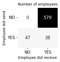
From the total number of 664 employees in the company, we learn that:

579 employees (87%) did not send any message despite receiving them.
Among those who did send messages (100% - 87% = 13% <–> 47 + 38 = 85 from 664), 47 of them did not receive any response.

Next I will take a look to the top 10 sender employees:

And here are the top centralities in the employee network:

Show code cell source Hide code cell source

# Create a multi directed graph
E = nx.MultiDiGraph()

# Add nodes
E.add_nodes_from(list(employees["id"]))

# Add metadata for each node
for node, (_, employee) in zip(E.nodes, employees.iterrows()):
    E.nodes[node]["department"] = employee["department"]
    E.nodes[node]["location"] = employee["location"]
    E.nodes[node]["age"] = employee["age"]

# E.nodes(data=True)

# Add messages as edges of the gragh
E.add_edges_from(
    [(message["sender"], message["receiver"]) for _, message in messages.iterrows()]
)

# Add metadata for each edge
for edge, (_, message) in zip(E.edges, messages.iterrows()):
    E.edges[edge]["timestamp"] = message["timestamp"]
    E.edges[edge]["message_length"] = message["message_length"]

# Degree centrality
degree_centrality_E = nx.degree_centrality(E)
dc_E = pd.DataFrame(degree_centrality_E.items(), columns=["node", "degree"]).set_index(
    "node"
)
dc_E = dc_E.div(dc_E.max())  # Normalize values

# Betweennness centrality
betweenness_centrality_E = nx.betweenness_centrality(E)
bc_E = pd.DataFrame(
    betweenness_centrality_E.items(), columns=["node", "betweenness"]
).set_index("node")
bc_E = bc_E.div(bc_E.max())  # Normalize values

# Join dataframe in the index
centralities = dc_E.join(bc_E)

# Sort values and get top
centralities = centralities.sort_values(by="degree", ascending=False)
top = 10
centralities_top = centralities[:top]

# Melt dataframe to plot in seaborn
centralities_melted = centralities_top.reset_index().melt(id_vars=["node"])

# Plot
fig, ax = plt.subplots(figsize=(6, 6))

sns.pointplot(
    x="variable",
    y="value",
    data=centralities_melted,
    ax=ax,
    hue="node",
    hue_order=centralities_melted["node"][:top],
    palette="Set1",
)

ax.grid(axis="y")
ax.set_axisbelow(True)
ax.tick_params(axis="y", which="major", labelsize=11)
ax.tick_params(axis="x", which="major", labelsize=11)
ax.set_title("Employee Centralities (top 10)", size=13)
ax.set_xlabel("", size=12)
ax.set_ylabel("Value (normalized)", size=12)
# Legend
h, l = ax.get_legend_handles_labels()


def identify_employee(id):
    dep = employees.loc[employees["id"] == int(id), :].iat[0, 1]
    loc = employees.loc[employees["id"] == int(id), :].iat[0, 2]
    return loc + " " + dep


ax.legend(
    h,
    [label + ": " + identify_employee(label) for label in l],
    bbox_to_anchor=(1.0, 0.5),
    loc="center left",
    fontsize=10,
    title="Employee",
)

sns.despine()

plt.show()

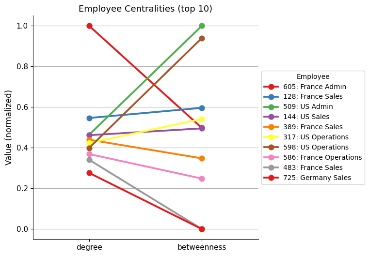
../_images/21ca3367a7fafa71b7d3953c483ae38152155266a327dcace26a793484eb0b90.png

The data indicates that the employees who send the most messages are also the ones with the most neighbors, meaning they occupy the top positions in terms of Degree Centrality. However, their position in the top ten varies when considering Betweenness Centrality, that is, their importance in the flow of information.

The employee 605 (from France Admin) stands out clearly for their activity. However, other employees are better connected, such as the 509 (US Admin).

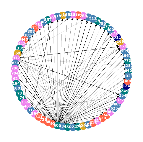
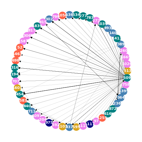
Below is the network diagram of the neighbors of employee 605 and employee 509, the top performers in terms of Degree Centrality and Betweenness Centrality, respectively.

../_images/cde0f91acf347d5b04b53cbc60c6f677afd31ba54a87ebefa4d7838a02444021.png

../_images/c0937cbe546d8bc6ba128545256148bb75ab6d04bd8c420b4594f39827d3f2d7.png

Conclusions#

Considering it in relative terms, that is, per employee, the Admin, Sales, and Operations departments of the US and France are the ones generating the bulk of the messages and are the most important in the flow of information within the organization. Comparatively, the rest of the departments seem less participative.

IT, Engineering, and especially Marketing barely communicate, and as for the countries, the UK stands out for its low activity.

It is striking the proportion of employees who did not send any messages (87%). And also, the fact that almost half of those who did send them, did not receive any response.

Regarding the most communicative employees, it is important to differentiate between the quantity of established connections and their importance in general terms of connectivity. In that sense, it was discovered that the employee who sent the most messages was surpassed by other employees who were initially less communicative when studying the relevance of those established contacts.

Employee Network Analysis

Contents

Employee Network Analysis#

The project#

The data#

Company#

Messages#

Between departments#

Between locations#

Departments in locations#

Employee network#

Conclusions#